FIRST: New Git Repository

To keep organized today we will start a fresh Git Repository that we will develop in for the next few weeks while working through spatial bioinformatics analyses.

Step 1: Create new Git repository on GitHub website.

Step 2: Create new project in RStudio + Version control with new repo

Step 3:

mkdir newrepo
cd newrepo

mkdir tmp #For stuff you do NOT want to commit to Git (e.g., climate dataa)
mkdir data # for data you do want to keep
mkdir R # for code
mkdir figures # for images and results files
echo "BIO331 Course Repository for Spatial Bioinformatics Unit" > README.md

## mkdir: cannot create directory ‘newrepo’: File exists
## mkdir: cannot create directory ‘tmp’: File exists
## mkdir: cannot create directory ‘data’: File exists
## mkdir: cannot create directory ‘R’: File exists
## mkdir: cannot create directory ‘figures’: File exists

Use the ‘data’ folder to save data files. Use the ‘R’ folder to hold your R scripts. Update the README.md file to describe what each file in your repository is for. Your repository contents will be graded at the end of this unit so be sure to perform regular commit/push operations to keep your progress up to date.

Species Distribution Modeling

As with virtually everything else the volume of data available to address biodiversity and ecology research questions is rapidly being collected and mobilized in massive databases. These large data aggregation projects pool data from hundreds or thousands of institutional collections and the work of many thousands of people collecting specimens and observational data on the occurrence of organisms.

Primary biodiversity data in the form of geographic point locality information and taxonomic identifications form the basis for modeling studies that seek to identify suitable habitat (often based on climate) for the species. These models have applications in current conservation practice to identify valuable habitat, but may also be projected into future climate to predict the potential impact of climate change on a species.

We will explore some data sources for GIS and Species Distribution Modeling (SDM) that are available in R. Then we will apply best practices to the machine learning algorithm Maxent to build predictions of species distributions.

READING: https://www.sciencedirect.com/science/article/pii/S1470160X18307635#f0010

R Packages: running list

For the next few lessons you will need: (UPDATE: These have all been installed locally)

install.packages('dismo') # Species Distribution Modeling tools
install.packages('raster') # R tools for GIS raster files
install.packages('spocc') # Access species occurrence data from GBIF/iNaturalist
install.packages('ENMeval') # Tuning SDMs
install.packages('mapr') # Quick mapping tools

Data Sources

We will be getting data for distribution modeling from:

Environmental Data: Continuous surfaces – > Raster data objects

Geographic data that are continuous across your study area can be represented as a gridded image-like data type known as a raster. These are basically really big 2 dimensional tables but with special attributes that help align the values in the matrix across the curved surface of Earth.

Important Terms:

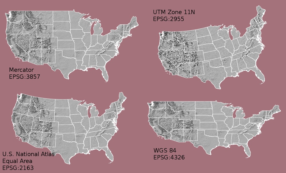
Resolution == The size of individual pixels in the raster grid. (alternate: The spatial area covered by each datapoint in the grid) Extent == The minimum and maximum longitude and latitude covered by a raster object Projection == The scheme used to translate 2D x,y/lat,long coordinates into 3D points on a spheroid earth. See illustration Layer == The data tables in a raster object. Each raster may consist of one layer or a stack of many layers

Our primary raster data will be climate from the WorldClim project.

Downloading climate data: WorldClim

We can download climate data for land masses except Antarctica using the ‘raster’ library and:

library(raster)

## Loading required package: sp

clim = getData('worldclim', var='bio', res=5) # Download the WorldClim Bioclim data for the world at a 5 arcminute resolution.

summary(clim)

## Warning in .local(object, ...): summary is an estimate based on a sample of 1e+05 cells (1.29% of all cells)

##            bio1    bio2    bio3       bio4    bio5    bio6    bio7    bio8
## Min.       -263      34       9     119.00     -59    -540      60    -242
## 1st Qu.     -40      87      21    3931.75     192    -272     243      88
## Median       86     110      32    8098.00     271     -76     343     157
## 3rd Qu.     226     135      52   12543.25     332      87     456     243
## Max.        314     210      94   22679.00     488     255     724     373
## NA's    5476792 5476792 5476792 5476792.00 5476792 5476792 5476792 5476715
##            bio9   bio10      bio11   bio12   bio13   bio14   bio15   bio16
## Min.       -451     -95    -488.00       0       0       0       0       0
## 1st Qu.    -150     117    -203.25     259      45       3      34     116
## Median       37     196     -19.00     492      78      11      54     209
## 3rd Qu.     221     265     168.00     929     150      25      81     396
## Max.        360     378     286.00    8967    1654     590     229    3821
## NA's    5476637 5476792 5476792.00 5476559 5476559 5476559 5476559 5476559
##           bio17   bio18   bio19
## Min.          0       0       0
## 1st Qu.      13      84      24
## Median       39     173      57
## 3rd Qu.      89     273     126
## Max.       1887    2936    3151
## NA's    5476559 5476792 5476792

summary(clim[[1]])

## Warning in .local(object, ...): summary is an estimate based on a sample of 1e+05 cells (1.29% of all cells)

##         bio1
## Min.    -265
## 1st Qu.  -40
## Median    87
## 3rd Qu.  227
## Max.     314
## NA's       0

See here for Bioclim variable definitions.

We are looking at ‘bio1’ above which is the mean annual temperature (MAT) value in Celsius degrees * 10.

Raster operations: Crop

If we want to ‘zoom in’ on a region of interest we can crop the raster just like a picture file. However, we must use the coordinates of the raster. In this case that is latitude and longitude in decimal degrees.

#define an 'extent' object.
#eastern US
ext = extent(-74, -69, 40, 45)

#crop
c2 = crop(clim, ext)
plot(c2[[1]]) # Basic plotting

Plot with ggplot

library(ggplot2)

c2_df = as.data.frame(c2, xy = TRUE)
head(c2_df)

ggplot() +
  geom_raster(data = c2_df, 
              aes(x = x, y = y, fill = bio1)) +
  coord_quickmap()

Improving the visualization: Color palettes and themes

Manual color palettes

First, set the base plot to a variable. ggplot functions can modify existing plot objects so we can use this ‘base’ image to try out new formatting.

base = ggplot() +
  geom_raster(data = c2_df, 
              aes(x = x, y = y, fill = bio1/10)) +
                coord_quickmap() +
  theme_bw()

base + scale_fill_gradientn(colours=c('navy', 'white', 'darkred'),
  na.value = "black")

Try Viridis colors

library(viridis)

## Loading required package: viridisLite

base + scale_fill_gradientn(colours=viridis(99), 
  na.value = "black")

base + scale_fill_gradientn(colours=magma(99), 
  na.value = "black")

Try ggsci colors. (https://cran.r-project.org/web/packages/ggsci/vignettes/ggsci.html)

library(ggsci) #for expanded colors
ggplot() +
  geom_raster(data = c2_df, 
              aes(x = x, y = y, fill = bio1), colours=viridis::viridis) +
                coord_quickmap() +
  theme_bw() + 
  scale_fill_gsea()

## Warning: Ignoring unknown parameters: colours

Raster values: Histogram

ggplot() +
  geom_histogram(data = c2_df, 
                 aes(x = bio1))

## `stat_bin()` using `bins = 30`. Pick better value with `binwidth`.

## Warning: Removed 1293 rows containing non-finite values (stat_bin).

ggplot() +
  geom_histogram(data = c2_df, 
                 aes(x = bio12)) #Histogram of Mean Precipitation values

## `stat_bin()` using `bins = 30`. Pick better value with `binwidth`.

## Warning: Removed 1293 rows containing non-finite values (stat_bin).

Next time: Vectors data, mining GBIF/iNaturalist, and ENMeval for distribution modeling

Homework: Plot MAP and Reading

Using the same raster climate data create a map of the Mean Annual precipitation in New England using variable ‘bio12’ (MAP in mm). Does your campus receive more or less precipitation each year than NYC. Save your code for today’s class AND the MAP plot to an R script and commit it to your new repository